Description
This is a quick python program I threw together to resolve one of the world’s most ancient and unresolved mysteries: blue/black or white/gold?
Dependencies
# We need these tools first to install the pip packages below:
sudo apt-get install build-essential python-dev python-pip python-imaging

pip install numpy
pip install matplotlib
Source
import numpy as np
import mpl_toolkits.mplot3d.axes3d as p3
import matplotlib.pyplot as plt
import colorsys
from PIL import Image
# (1) Import the file to be analyzed!
img_file = Image.open("thedress.jpg")
img = img_file.load()
# (2) Get image width & height in pixels
[xs, ys] = img_file.size
max_intensity = 100
hues = {}
# (3) Examine each pixel in the image file
for x in xrange(0, xs):
for y in xrange(0, ys):
# (4) Get the RGB color of the pixel
[r, g, b] = img[x, y]
# (5) Normalize pixel color values
r /= 255.0
g /= 255.0
b /= 255.0
# (6) Convert RGB color to HSV
[h, s, v] = colorsys.rgb_to_hsv(r, g, b)
# (7) Marginalize s; count how many pixels have matching (h, v)
if h not in hues:
hues[h] = {}
if v not in hues[h]:
hues[h][v] = 1
else:
if hues[h][v] < max_intensity:
hues[h][v] += 1
# (8) Decompose the hues object into a set of one dimensional arrays we can use with matplotlib
h_ = []
v_ = []
i = []
colours = []
for h in hues:
for v in hues[h]:
h_.append(h)
v_.append(v)
i.append(hues[h][v])
[r, g, b] = colorsys.hsv_to_rgb(h, 1, v)
colours.append([r, g, b])
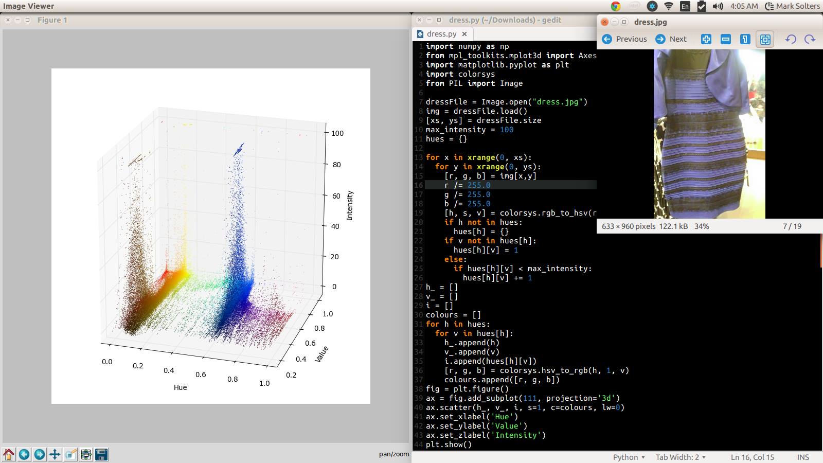
# (9) Plot the graph!
fig = plt.figure()
ax = p3.Axes3D(fig)
ax.scatter(h_, v_, i, s=5, c=colours, lw=0)
ax.set_xlabel('Hue')
ax.set_ylabel('Value')
ax.set_zlabel('Intensity')
fig.add_axes(ax)
plt.show()
Breakdown
Read Each Pixel’s Color
Basically, we are going to scan a given image file, pixel by pixel. For each pixel, we will determine the color in (r, g, b).
# (1) Import the file to be analyzed!
img_file = Image.open("thedress.jpg")
img = img_file.load()

# (2) Get image width & height in pixels
[xs, ys] = img_file.size
max_intensity = 100
hues = {}

# (3) Examine each pixel in the image file
for x in xrange(0, xs):
  for y in xrange(0, ys):
    # (4)  Get the RGB color of the pixel
    [r, g, b] = img[x, y]

    # (5)  Normalize pixel color values
    r /= 255.0
    g /= 255.0
    b /= 255.0
Change Colorspaces
Then we map from (r, g, b) to (h, s, v) (hue, saturation and value). We are doing this because the HSV model give us a nice “rainbow” in the H dimension, essentially sorting the colors from lowest wavelength to highest.
    # (6)  Convert RGB color to HSV
    [h, s, v] = colorsys.rgb_to_hsv(r, g, b)
Integrate Saturation
We have a 3-dimensional color space, and for some subset of points in this space, we have assigned a value corresponding to the number of pixels in the image that share that color. Those are 4 dimensions we need to somehow plot!
To simplify, we are going to marginalize over the saturation parameter. We’re essentially going to integrate over s, from 0 to 1, for every pair of (h, v) that appears in our image.
For every (h, v) pair in our color space that represents a non-zero number of pixels, we take the sum of all pixels that share those (h, v) values, regardless of saturation. Now we have something that can be represented using 3 dimensions:
hues(h, v) = i
The idea of this hues structure is that for any given (h, v), hues[h][v] represents the number of pixels appearing in the image with those hue and value parameters. In this application we have set a maximum value for any i because outliers will distort the Z-axis of the graph. Therefore, any colours that appear in more pixels than max_intensity will appear as clusters on the roof of our chart.
    # (7)  Marginalize s; count how many pixels have matching (h, v)
    if h not in hues:
      hues[h] = {}
    if v not in hues[h]:
      hues[h][v] = 1
    else:
      if hues[h][v] < max_intensity:
        hues[h][v] += 1
Linearize Data
Having arrived at this hues object, we need to now construct three separate arrays, for h, v, and i. We also keep a fourth array, called colours. This allows us to tag each point in the chart with the color it represents (assume saturation=1.0). The idea is that picking an index k, the value of (h[k], s[k], v[k]) is the color of data point k; in addition, its RGB equivalent is located in colours[k].
# (8)   Decompose the hues object into a set of one dimensional arrays we can use with matplotlib
h_ = []
v_ = []
i = []
colours = []

for h in hues:
  for v in hues[h]:
    h_.append(h)
    v_.append(v)
    i.append(hues[h][v])
    [r, g, b] = colorsys.hsv_to_rgb(h, 1, v)
    colours.append([r, g, b])
This step is necessary because that’s how the Axes3D.scatter() method’s arguments are setup.
Render
# (9)   Plot the graph!
fig = plt.figure()
ax = p3.Axes3D(fig)
ax.scatter(h_, v_, i, s=5, c=colours, lw=0)

ax.set_xlabel('Hue')
ax.set_ylabel('Value')
ax.set_zlabel('Intensity')
fig.add_axes(ax)
plt.show()